In my previous post, I described how I built a Singularity container with an editable fastai2 installation for use in the new iteration of their Deep Learning Part 1 course (aka ‘part1-v4’), which is currently on-going.
In this post I would like to share (and record for my own future reference!) my exploratory use of fastai2 on a dataset/challenge that is of interest in the built environment, which is an obvious area of focus for my company Arup.
The dataset is from the PEER Hub ImageNet (PHI) Challenge 2018 1 2, which is apparently the first image-based structural damage recognition competition, with a large image dataset (now called Φ-Net) relevant to the field of structural engineering. PEER designed a total of eight detection tasks 2 to contribute to the establishment of automated vision-based structural health monitoring. Using fastai2, I explored a few of these tasks, and will use Task 1 as an example in this post.
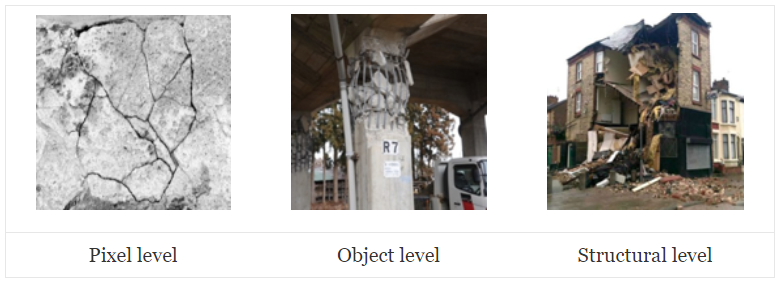
Task 1 – Scene level – Three classes (pixel/object/structural):
Looking at the data
For Task 1, PEER provided 17424 labelled images, marked as one of the three classes – pixel/object/structural. I was not part of the original PHI Challenge back in 2018, and do not actually know how PEER provided the dataset at the time. The data that I have (courtesy of my colleagues’ entry in the PHI Challenge) is a set of numpy .npy files, which contain the bitmap RGB data with standard resolution 224 × 224px, and their respective class labels. The test set images are also available (along with the sample_submission.csv for the original challenge entry submission), but I do not have the corresponding labels (i.e. the ‘answers’) for the test set:
ylee@hpc01 Task1 ]$ ls
sample_submission.csv  X_test.npy  X_train.npy  y_train.npy
The first thing is obviously to have a look at the data. This means loading it using numpy, where the shape of (17424, 224, 224, 3) indicates that it should be 17424 images of 224px sides with three channels (RGB).
import numpy as np

data = np.load('X_train.npy')
y = np.load('y_train.npy')

print(data.shape, y.shape)
(17424, 224, 224, 3) (17424,)
We can confirm the image data by using PIL to create an image from the first item, and showing it inline in Jupyter Notebook:
from PIL import Image

im = Image.fromarray(data[0])
im
I prefer to have image data in the form of actual image files, as it makes it possible to easily look at the data just by using image viewers or thumbnail view in a file manager. PIL can be used to save the dataset back into bitmap .bmp files. I chose to output filenames in the format of num_pX.bmp, where num is the item number [0 to 17423] and X is the class ID (0 = pixel; 1 = object; 2 = structural).
for i in range(len(data)):
    fname = '%05d_p%s.bmp' % (i, y[i])
    im = Image.fromarray(data[i])
    im.save(fname)
To make it easier for data-loading in fastai2, I created three subfolders and just moved the images by class into the respective folders. Incidentally, this actually made it easier later on, when I started to put in my own ‘corrections’ to the PHI training data set labels. I also quickly checked how many images there are for each class.
ylee@hpc01 bmp ]$ mkdir p0
ylee@hpc01 bmp ]$ mv *_p0.bmp ./p0/
ylee@hpc01 bmp ]$ ls ./p0/ | wc -l
5879
ylee@hpc01 bmp ]$ mkdir p1
ylee@hpc01 bmp ]$ mv *_p1.bmp ./p1/
ylee@hpc01 bmp ]$ ls ./p1/ | wc -l
5713
ylee@hpc01 bmp ]$ mkdir p2
ylee@hpc01 bmp ]$ mv *_p2.bmp ./p2/
ylee@hpc01 bmp ]$ ls ./p2/ | wc -l
5832
Looks like the 17424 images were roughly evenly split into the three classes, i.e. no real need to worry about imbalanced data set. Note that the above could have been done within Python in Jupyter Notebook, but I am in the shell terminal a lot anyways, so I just did it in terminal.
Now that the data is in the form of .bmp files, with subfolders indicating their respective labels, it is straightforward to load into fastai2.
path = Path('/data/phi_challenge/task1/bmp')

path.ls()
(#3) [Path('/data/phi_challenge/task1/bmp/p0'),
Path('/data/phi_challenge/task1/bmp/p1'),
Path('/data/phi_challenge/task1/bmp/p2')]
Using fastai2’s very convenient get_image_files function to get all the image filenames (in this case, they are .bmp files):
fns = get_image_files(path)
fns
(#17424) [Path('/data/phi_challenge/task1/bmp/p0/00000_p0.bmp'),
Path('/data/phi_challenge/task1/bmp/p0/00002_p0.bmp'),
Path('/data/phi_challenge/task1/bmp/p0/00006_p0.bmp'),
Path('/data/phi_challenge/task1/bmp/p0/00007_p0.bmp'),
Path('/data/phi_challenge/task1/bmp/p0/00009_p0.bmp'),
Path('/data/phi_challenge/task1/bmp/p0/00011_p0.bmp'),
Path('/data/phi_challenge/task1/bmp/p0/00012_p0.bmp'),
Path('/data/phi_challenge/task1/bmp/p0/00016_p0.bmp'),
Path('/data/phi_challenge/task1/bmp/p0/00017_p0.bmp'),
Path('/data/phi_challenge/task1/bmp/p0/00019_p0.bmp')...]
Followed by another useful function, verify_images, to check for invalid image files. In this case, it returned zero item, i.e. all 17424 images were okay – expected, since they were written into image files by PIL previously!
failed = verify_images(fns)
failed
(#0) []
Then, I can create a fastai2 DataBlock with the labelled data set. For more information on the fastai2 DataBlock API, have a look at this great blog post from Zach Mueller.
phi1 = DataBlock(
    blocks=(ImageBlock, CategoryBlock),
    get_items=get_image_files,
    splitter=RandomSplitter(valid_pct=0.2),
    get_y=parent_label,
    batch_tfms=aug_transforms())

dls = phi1.dataloaders(path)
- The
blocksfor this data set are images (independent variable) and category (dependent variable) i.e. the label. - The data items can be obtained from the same
get_image_filesfunction used above. - I used
RandomSplitterto create a validation set with 20% of randomly chosen training data. - The
y(dependent) variable can be obtained from the subfolder name, i.e. ‘parent_label’ of the image filenames. - This is just for quick exploration, so I just used the fastai2 defaults for data augmentation, passing the transform definitions from
aug_transformsto be applied onto the data batches.
After that, a DataLoader (PyTorch-style) is created from the path containing my data, using the DataBlock definition above.
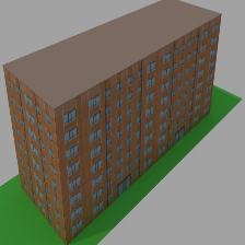
Now I can do a quick visual check on the data, by showing a single batch of the images with their labels. The default batch size is 64, but I just need to see a few of the images to spot-check for any problem, so I asked for 16 in a batch to be shown.
dls.valid.show_batch(max_n=16)
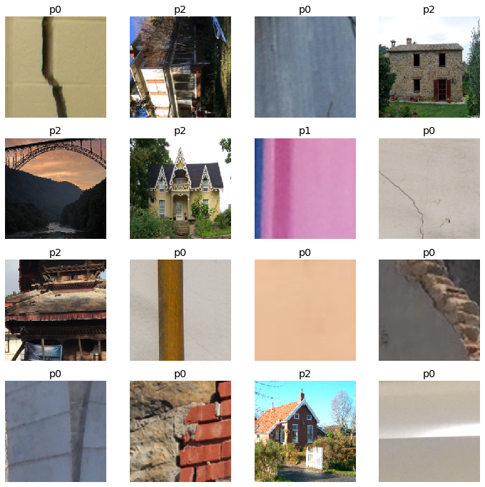
Looks reasonable, with pixel-level labelled as p0 (e.g. a crack on a wall), object-level as p1 (only one item shown above, looks like part of a wall/column?), and structure-level as p2 (e.g. a whole house/building/bridge). There seems to be a p2 image that was wrongly rotated by 90°, but I’ll just leave it for now, unless it turns out to be a problem when looking at the trained model and its predictions and interpretations later.
Create and train model
From here, it is very easy to create a standard CV deep learning CNN learner, with the DataLoader (defined above) and a pretrained model (i.e. the now-ubiquitous “transfer learning” method). Here I used a pretrained ResNet34 model, asking for an additional KPI metric of error rate during training.
Then, I asked for the model to be trained and fine-tuned for five epochs, using the default fastai2 hyperparameters without thinking too much about it (since it’s just for exploring~).
learn = cnn_learner(dls, resnet34, metrics=error_rate)
learn.fine_tune(5)
| epoch | train_loss | valid_loss | error_rate | time |
|---|---|---|---|---|
| 0 | 0.522718 | 0.320116 | 0.124569 | 00:32 |
| epoch | train_loss | valid_loss | error_rate | time |
|---|---|---|---|---|
| 0 | 0.320330 | 0.233091 | 0.093571 | 00:52 |
| 1 | 0.262438 | 0.225992 | 0.098163 | 00:49 |
| 2 | 0.210474 | 0.198712 | 0.080941 | 00:46 |
| 3 | 0.143000 | 0.205004 | 0.076636 | 00:45 |
| 4 | 0.102853 | 0.202703 | 0.073192 | 00:44 |
As shown above, with just the initial training of the ‘head’ of the ResNet34 model (with the original model parameters pretrained on ImageNet), it was already achieving an error rate of just 12.5%, which is not too shabby. Note that it is recommended and sensible to first try and establish a simple ‘baseline’ for sanity check and basic benchmark, but I did not do that here (sorry!).
During five more epochs of fine-tuning, we can see that both training loss and validation loss continue to decrease, i.e. the model is ‘learning’ successfully. The ever-reducing validation loss indicates that the model is not quite suffering from the dreaded ‘overfitting’ yet. At the end of a total of just six epochs of training, the model has an error rate (‘judged’ on the random 20% validation set) of 7.3%, or in other words, it is 92.7% accurate in differentiating between the three classes. That’s pretty good-going, with just ~5 minutes of training (albeit on an NVIDIA Tesla V100…)!
I can then show the confusion matrix to see where the errors are made:
interp = ClassificationInterpretation.from_learner(learn)
interp.plot_confusion_matrix()
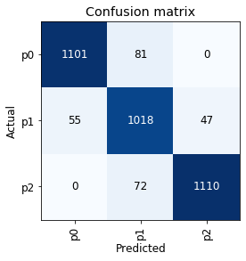
The confusion matrix looks reasonable, in that the model did not ‘skip’ a level in mistaking p0 as p2 or vice versa. As an aside, this might mean that there will not be much benefit in trying an ‘ordinal regression’ approach for this classification exercise (though it might still be worth trying, something for another time, perhaps).
In addition to confusion matrix, it is also useful to plot the images that gave the top losses, to see where/what the model was most inaccurate with:
interp.plot_top_losses(36)
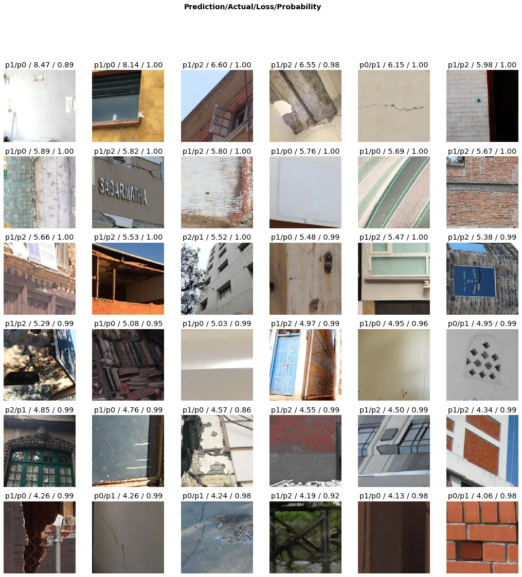
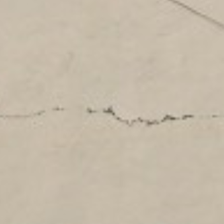
This is where I cannot say that I agree with some of the labels in the data set… For example, in the grid above, the second from right image in the first row (shown again below) is labelled p1 (i.e. object-level), but it sure looks like a p0 (i.e. pixel-level) to my human eyes, in agreement with the trained model’s prediction!
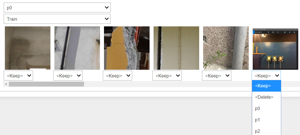
For cases like this, with fastai2 it is possible to quickly ‘correct’ the data within Jupyter Notebook, taking and modifying some functions from the part1-v4 course notebooks, which uses ipywidgets to provide a graphical UI for picking actions. I can call the ImageClassifierCleaner function on the CNN learner, and display the UI to pick the correcting ‘actions’ for images of interest:
cleaner = ImageClassifierCleaner(learn)
cleaner
For data tracking purposes, I modified the ‘correction’ actions from the original part1-v4 notebook, so that instead of actually deleting unwanted training data images (with the unlink function), it renames the unwanted .bmp file to .deleted instead, which means that when I retrain a model with the cleaned data the ‘deleted’ files will not be picked up by the get_image_files function (see above). Because of the way I formed the .bmp filenames when writing out the original .nyp data into .bmp images, it is very easy to see which images have been discarded (i.e. renamed to .deleted), and which images have had their labels corrected (e.g. nnnnn_p1.bmp being moved into the p0 subfolder) if I want to trace back the changes/corrections that I made.
for idx in cleaner.delete():
#     cleaner.fns[idx].unlink()
    delname = "%s/%s.deleted" % (str(cleaner.fns[idx].parent), cleaner.fns[idx].name[:-4])
    shutil.move(str(cleaner.fns[idx]), delname)
for idx,cat in cleaner.change(): shutil.move(str(cleaner.fns[idx]), path/cat)
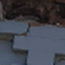
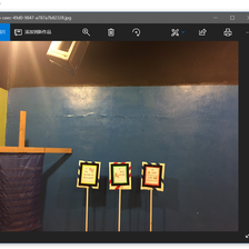
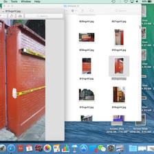
In a few rounds of quick training, plotting top losses, and running ImageClassifierCleaner, I ended up deleting a few images as shown below, where they look like strange computer screenshots instead of actual photos:
I also ‘corrected’ (by my interpretation) the labels for about 120 images, which is only ~0.7% of the data set, but I think it’s always useful to have more accurately labelled data, especially when it’s so easy to correct them within the notebooks!
Results and quick comparison
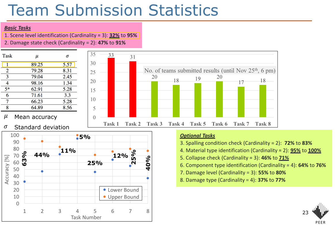
After these corrections, in about 30 minutes of training across four quick experimental notebooks, the best error rate I got was around 6.6% with a pretrained ResNet50 model, or a 93.4% accuracy. Looking at this pdf, the 2018 PHI Challenge winners achieved a test set accuracy of 95% for Task 1, using ensembles of trained models. The mean accuracy for Task 1 was 89%, so my numbers (caveat below) are between the mean and the winner (closer to the winner), which is not too bad : )
Some thoughts on these:
- For the amount of work put into these quick exploration and training, I am quite happy with the accuracy of 93% vs. the winning 95% (back in 2018), though obviously note that a difference of ~18 months is aaaaaaaages in the Deep Learning world in terms of improvements in techniques, best practices, and results metrics!
- To some, an accuracy difference of 2% might not sound like much, but actually, the winning entry in 2018 (5% error) is 2 percentage points better than my 7% error, i.e. it’s 2/7 × 100 = 29 percent better!
- As I only have the validation-set accuracy (of 20% randomly chosen from the labelled data) and do not have the test-set ‘answers’, it is not really a like-for-like comparison with the PHI Challenge numbers, though I think it’s likely still indicative.
- I have only used a single ResNet model, and I am not sure whether (or how much) ensembles of models can help with my numbers, noting that ensembles seemed to have significantly boosted the PHI Challenge 2018 winning entries, so it is definitely worth looking into.
- I wonder if there are higher resolution images available for the same data set, and whether (or how much) that might help. I used 224 × 224px images that I had to hand, but there might be better quality, higher-resolution images available. It seems like the great people at PEER have now made their Φ-Net dataset available for download, but I have not downloaded or looked at it yet – maybe this is the same 224px data that I already have.
- fastai2 has made it very easy for me to load in the data, explore the data visually, create CNN models with pretrained architectures, interpret training results, and even quickly correct mislabelled (I think) data for retraining. As always, kudos to the great people at fast.ai, including the vibrant user community there.
Citations:
-
Gao, Y. and Mosalam, K. M. (2019). PEER Hub ImageNet (Φ-Net): A large-scale multi-attribute benchmark dataset of structural images, PEER Report No.2019/07, Pacific Earthquake Engineering Research Center, University of California, Berkeley, CA. ↩
-
Gao, Y., & Mosalam, K. M. (2018). Deep transfer learning for image-based structural damage recognition. Computer-Aided Civil and Infrastructure Engineering, 33(9), 748-768. ↩ ↩2